 , or one-in-a-billion, is the famed number given for the maximum probability of a catastrophic failure, per hour of operation, in life-critical systems like commercial aircraft. The number is part of the folklore of the safety-critical systems literature; where does it come from?
First, it’s worth noting just how small that number is. As pointed out by Driscoll et al. in the paper, Byzantine Fault Tolerance, from Theory to Reality, the probability of winning the U.K. lottery is 1 in 10s of millions, and the probability of being struck by lightening (in the U.S.) is  more than a 1,000 times more likely than
So where did come from? A nice explanation comes from a recent paper by John Rushby:
If we consider the example of an airplane type with 100 members, each flying  hours per year over an operational life of 33 years, then we have a total exposure of about 107 flight hours. If hazard analysis reveals ten potentially catastrophic failures in each of ten subsystems, then the “budget” for each, if none are expected to occur in the life of the fleet, is a failure probability of about per hour [1, page 37]. This serves to explain the well-known requirement, which is stated as follows: “when using quantitative analyses. . . numerical probabilities. . . on the order of per flight-hour. . . based on a flight of mean duration for the airplane type may be used. . . as aids to engineering judgment. . . to. . . help determine compliance” (with the requirement for extremely improbable failure conditions) [2, paragraph 10.b].
[1] E. Lloyd and W. Tye, Systematic Safety: Safety Assessment of Aircraft Systems. London, England: Civil Aviation Authority, 1982, reprinted 1992.
[2] System Design and Analysis, Federal Aviation Administration, Jun. 21, 1988, advisory Circular 25.1309-1A.
(By the way, it’s worth reading the rest of the paper—it’s the first attempt I know of to formally connect the notions of (software) formal verification and reliability.)
So there a probabilistic argument being made, but let’s spell it out in a little more detail. If there are 10 potential failures in 10 subsystems, then there are  potential failures. Thus, there are
  possible configurations of failure/non-failure in the subsystems. Only one of these configurations is acceptable—the one in which there are no faults.
If the probability of failure is  then the probability of non-failure is
  So if the probability of failure for each subsystem is
  then the probability of being in the one non-failure configuration is

We want that probability of non-failure to be greater than the required probability of non-failure, given the total number of flight hours. Thus,

which indeed holds:

is around 
Can we generalize the inequality? The hint for how to do so is that the number of subsystems ( ) is no more than the overall failure rate divided by the subsystem rate:

This suggests the general form is something like
Subsystem reliability inequality: 
where 
 and
and  are real numbers,
 and
and 
Let’s prove the inequality holds. Joe Hurd figured out the proof, sketched below (but I take responsibility for any mistakes in it’s presentation). For convenience, we’ll prove the inequality holds specifically when  but the proof can be generalized.
First, if  the inequality holds immediately. Next, we’ll show that

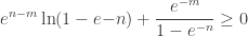
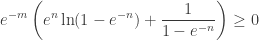
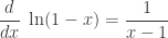
is monotonically non-decreasing with respect to  by showing that the derivative of its logarithm is greater or equal to zero for all
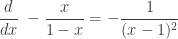
  So the derivative of its logarithm is

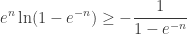
We show
iff
and since 
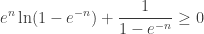
iff
Let  , so the range of
  is
is 

Now we show that in the range of , the left-hand side is bounded below by the right-hand side of the inequality.

and

Now taking their derivatives
and
Because  in the range of , our proof holds.
The purpose of this post was to clarify the folklore of ultra-reliable systems. The subsystem reliability inequality presented allows for easy generalization to other reliable systems.
Thanks again for the help, Joe!
Tags: 10^-9, probability, reliability, safety-critical systems
This entry was posted on January 24, 2010 at 11:00 pm and is filed under Fault Tolerance, Hardware. You can follow any responses to this entry through the RSS 2.0 feed.
You can leave a response, or trackback from your own site.

January 24, 2010 at 11:22 pm |
Much simpler way of doing the math: The probability that something has failed is less than or equal to the expected number of things which have failed. If you have 100 events which occur, each with probability 10^-9, the average number of them which are occuring at any point in time is 100 * 10^-9 = 10^-7; so you immediately have that the probability that one or more is occuring is less than or equal to 10^-7.
No logarithms required. (Also, using this argument you don’t need to make the assumption that failures are independent of each other, which you implicitly do.)
January 25, 2010 at 7:52 am |
Thanks for the note. You note that
I believe you are computing the expected value here—for example, if I flip a fair coin three times, I expect to see heads 3 * 0.5 = 1.5 times. The probability of one or more heads is computed by .
.
January 25, 2010 at 8:06 am
The expected number of events is
sum(n * P(there are exactly n events))
i.e. since the number of events is discrete, it is
0 * P(exactly 0 events) + 1 * P(exactly 1 event) + 2 * P(exactly 2 events) + …
This is greater than
1 * P(exactly 1 event) + 1 * P(exactly 2 events) + …
which is equal to P(>=1 event)
January 25, 2010 at 1:21 am |
Did you mean n=m for the base case, not n=0? The LHS goes to 0 if n=0, and anyway we’re not interested in the case where each component is *more* unreliable than we want the system to be.
January 25, 2010 at 2:20 am |
Social comments and analytics for this post…
This post was mentioned on Twitter by donsbot: Lee Pike’s post on one-in-a-billion critical system failures, https://leepike.wordpress.com/2010/01/24/10-9/…
January 25, 2010 at 5:27 am |
It’s not clear to me that (1 – e^{-n})^{e^{n-m}} >= 1 – e^{-m} holds immediately if n = 0. Substituting in, e^{-n} becomes e^0 becomes 1, and the left-hand side of the inequality collapses to 0. This leaves 0 >= 1 – e^{-m}, which rearranges to e^{-m} >= 1, then -m >= 0, and finally m <= 0. Judging by the previous part of your post, m is typically positive, which suggests a problem. What have I missed?
January 25, 2010 at 8:05 am |
Neil, Ganesh—typo! Thanks for the catch. I changed the post so that .
.
January 25, 2010 at 5:16 pm |
[…] 10 to the -9 , or one-in-a-billion, is the famed number given for the maximum probability of a catastrophic failure, per hour of […] […]
February 2, 2010 at 1:00 pm |
You only proved that f(n)=(1 – e^{-n})^{e^{n-m}} is non-decreasing. As a consequence, f(n) >= f(m) = 1 – e^{-m} IF n >= m. Otherwise, if n <= m the proof breaks and you have the reverse: f(n) = 1-rx
for 0 <= x = 1? Which can be proven (similarly) by noting that f(x) = (1-x)^r – 1 + rx, then f'(x) >= 0 for all 0 <= x = 0 -> f(x) >= 0 (by mean value theorem).
With the above, x = C^{-n}, r = C^{-m+n}, and you recover your result (only if C^n >= C^m which is to say r>=1).
February 2, 2010 at 11:51 pm |
Thanks—another typo. I think I’ve fixed the assumptions now.
February 3, 2010 at 3:25 am |
The probability of winning the U.K. lottery is 1 in 10s of millions, and the probability of being struck by lightening (in the U.S.) is 1.6 \times 10^{-6}, about a 1,000 times more likely. 1 in 10s of millions is 10^(-7) so the probability of being struck by lightning should be 6 times more likely.
February 3, 2010 at 8:42 pm |
Sorry for the ambiguity—I meant that is 1,000 times more than
  I’ve updated the post to make it clear.
February 3, 2010 at 10:50 am |
My original comment got munched up somehow. My point was that this whole thing is identical to: for
for  , which you can prove slightly more directly (no logs) by the same method: show that
  is non-decreasing when
  and note