Viva La Resistance! A Resistance Game Solver

Update (Feb142016): see bottom for an improved strategy.

The Game

At a December workshop, I played The Resistance, a game in which there are two teams, the resistance and the spies. The spies know everyone’s identity; each resistance player knows only one’s own. Overall, the goal of the spies is to remain undetected; the goal of the resistance is to discover who the spies are.

Play proceeds in rounds in which a player nominates a subgroup to go on a “mission”. The nomination is then voted on. If the vote succeeds, every member of a mission plays either a “success” or “failure” card for the mission. One or two failure cards (depending on the mission size) causes the mission to fail. The cards played in a mission are public, but it is secret who played which card. (If the vote fails, the next player nominates a subgroup.)

The spies’ goal is to fail missions without being detected, and the resistance goal is to have missions succeed. So the spies generally wish to play failure cards while in a mission. Furthermore, spies always want some spy in the mission to spoil it. The resistance wants no spies to go on missions. The problem for the resistance is that when a mission fails, they know one or more of the subgroup is a spy, they just don’t know which one.

The spies win the game if they can cause three missions to fail before the resistance can cause three missions to succeed.

The game is simple but engaging, and similar in spirit to the game Mafia (Werewolf).y

The Problem

I played the game with computer scientists from the top universities and research labs. We debated strategy and were generally pretty bad at the game, despite having a lot of fun. In particular, the spies seemed to win a lot.

The problem is: what is the optimal approach to game play?

The Approach

The problem is a great fit for Bayesian Analysis. In each round, we learn partial information about the players from the group outcome. Only spies play failure cards. We can use that information to update our believe in the probability that a player is a spy.

Suppose there are four players, and two spies. Initially each player has the same probability of being a spy, . Now suppose that go on a mission, and return the set of cards . How do we update the spy probabilities of the group?

Bayes Theorem states that

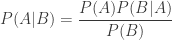
In our case, “A” is the event that a particular player is a spy, and “B” is the event that we we observed a particular set of mission cards. We wish to compute , the updated probability that a player is a spy given the cards played in the mission.

So for each mission, we apply Bayes’ Theorem to each player, including the players not in the mission—if the spy probabilities increase (or decrease) for the mission players, then they decrease (or increase) for the non-mission players.

From the cards , we know that two of  are spies (and so is definitely not a spy, since there are two spies, total). Let’s compute the updated spy probability for player .

, the original spy probability for player (or any other player). To calculate , we first determine every possible assignment of players in the mission to spies and non-spies (there are such assignments). In the mission, there are three possibilities:

1. spies
2. spies
3. spies

For each combination, we multiply the probabilities for the assignments. So in case (1), we have

for assigning players  and  to being spies and c to being a non-spy. Then we sum the probabilities for all three combinations. In our example, we get

So .

To compute P(B|A), we assume that player a is a spy, and now recompute the probability that contains the remaining one spy. Using the same approach as for computing , we get . Now we can apply Bayes’ Theorem:

So player’s a probability of being a spy shot up to 0.66, and so did player b’s and c’s.

Player ‘s spy probability drops to 0. The updated spy probabilities for any player not in the mission can be computed just as we did for the mission players, except we take the total number of spies and subject the number of failure cards observed. In this case, however, since we know all the spies were in the group, ‘s spy probability must be 0. (Another way of thinking about it is that there is an invariant that the sum of the player’s spy probabilities must always be the total number of spies in the group.)

The Strategies

How should the game be played by the resistance and spies, respectively, to increase the odds of winning?

For the resistance, picking the players the least likely to be spies is optimal. Let’s call this the pick-lowest strategy.

One possible optimization is to always pick yourself in a mission. The rational is that you know if you are part of the resistance, and you pick yourself for a mission, then you have at least one guaranteed non-spy. So even if your probability of being a spy as known to the group is higher than others, you have perfect knowledge of yourself. Let’s call this the pick-myself strategy,

For the spies, there are a few options. By default, the spies could always play a failure card (fail-always). But a spy might also play a success card to avoid detection; doing so is especially advantageous in the early rounds; one strategy is to never fail the first round (succeed-first). If the spies can collude to ensure only one plays a failure card during a mission, that provides the least amount of information to the resistance (fail-one).

There are other strategies and other combinations of strategies, but this is a good representative sample.

Which are the best strategies?

Findings

To discover the best strategies, we use Monte-Carlo simulations on the strategies over each number of players (with different number of players, there are different number of spies and missions). I found a few interesting results:

• The best chance of wining for the resistance, and the closest odds between the resistance and spies, is with six players. At six players, the resistance has a 30-40% chance of winning under different strategies. The worst configuration is eight players, with not more than a 14% chance of winning for the resistance. During actual game play, it seemed that the odds favored the spies.
• The best strategy for the resistance is the pick-lowest strategy. The strategy may be counter-intuitive, but consider this: the pick-myself strategy provides the spies an opportunity to always include themselves in a mission when picking a mission. The pick-myself strategy is an instance of a local maxima (i.e., local knowledge of knowing yourself to be part of the resistance) that is non-optimal.
• Moreover, voting becomes a no-op. The game includes a voting round in which players vote on the proposed players for a mission. But If the resistance agrees on an optimal strategy, any deviation from the strategy by a player is because the player is a spy. If the person does deviation, the resistance votes against it (and resistance outnumber spies, so will win the vote), and we now have complete assurance the proposer is a spy. The spies have no choice but to follow the optimal strategy of the resistance.
• Of the spy strategies listed above, the best is the fail-one strategy, which is intuitive. The succeed-first strategy is another example of a local maxima that is non-optimal; while it protects that particular spy from detection, it is more valuable for the spies in general to fail the mission.

The related Mafia game has some analytical results, giving bounds on (their version of) the resistance to spies. I have not done that, nor have I done Monte-Carlo analysis to determine what proportion of resistance and spies and mission sizes gives a more even chance of winning. In Mafia, it is noted that in actual game play, the resistance wins more often than simulations/analytical analysis would suggest, with different attributions (e.g., people are bad at lying over iterative rounds).

Play Along at Home

I have implemented the Bayesian solver in a webserver hosted on Amazon Web Services. You can use the solver when playing with others.

http://ec2-54-173-249-238.compute-1.amazonaws.com/

An easier-to-remember link is http://tiny.cc/theresistance1.

If you want to run Monte Carlo simulations, you will have to download the code and run it locally, however.

Implementation

https://github.com/leepike/theresistance

Update (Feb142016)

It has been pointed out by Eike Schulte in the comments and Iavor Diatchki that by including some additional information, the strategy might be improved. This is indeed the case. The intuition is that if a group has previously included a spy, that group should not be selected again, even if it is the lowest probability group. For example, with five players, consider the following rounds:

• Round 0: players [0,1] are selected and there is one fail card.
• Round 1: players [2,3,4] are selected and there is one fail card.
• Round 2: players [2,3] are selected and there are no fail cards.

At this point, players [0,1] have a 0.5 probability of being a spy and players [2,3,4] have a 1/3 probability. So in round 3, we do not want to select players [2,3,4] even if they have the lowest probabilities. So we select a group with the lowest spy probability that has not already included a spy. The server has been updated to include this strategy. The strategy does better; for example, at 6 players, we have just over a 50% chance of winning!

SmartChecking Matt Might’s Red-Black Trees

Matt Might gave a nice intro to QuickCheck via testing red-black trees recently. Of course, QuickCheck has been around for over a decade now, but it’s still useful (if underused–why aren’t you QuickChecking your programs!?).

In a couple of weeks, I’m presenting a paper on an alternative to QuickCheck called SmartCheck at the Haskell Symposium.

SmartCheck focuses on efficiently shrinking and generalizing large counterexamples. I thought it’d be fun to try some of Matt’s examples with SmartCheck.

The kinds of properties Matt Checked really aren’t in the sweet spot of SmartCheck, since the counterexamples are so small (Matt didn’t even have to define instances for shrink!). SmartCheck focuses on shrinking and generalizing large counterexamples.

Still, let’s see what it looks like. (The code can be found here.)

SmartCheck is only interesting for failed properties, so let’s look at an early example in Matt’s blog post where something goes wrong. A lot of the blog post focuses on generating sufficiently constrained arbitrary red-black trees. In the section entitled, “A property for balanced black depth”, a property is given to check that the path from the root of a tree to every leaf passes through the same number of black nodes. An early generator for trees fails to satisfy the property.

To get the code to work with SmartCheck, we derive Typeable and Generic instances for the datatypes, and use GHC Generics to automatically derive instances for SmartCheck’s typeclass. The only other main issue is that SmartCheck doesn’t support a `forall` function like in QuickCheck. So instead of a call to QuickCheck such as

> quickCheck (forAll nrrTree prop_BlackBalanced)


We change the arbitrary instance to be the nrrTree generator.

Because it is so easy to find a small counterexample, SmartCheck’s reduction algorithm does a little bit of automatic shrinking, but not too much. For example, a typical minimal counterexample returned by SmartCheck looks like

T R E 2 (T B E 5 E)


which is about as small as possible. Now onto generalization!

There are three generalization phases in SmartCheck, but we’ll look at just one, in which a formula is returned that is universally quantified if every test case fails. For the test case above, SmartCheck returns the following formula:

forall values x0 x1:
T R E 2 (T B x1 5 x0)


Intuitively, this means that for any well-typed trees chosen that could replace the variables x0 and x1, the resulting formula is still a counterexample.

The benefit to developers is seeing instantly that those subterms in the counterexample probably don’t matter. The real issue is that E on the left is unbalanced with (T B E 5 E) on the right.

One of the early design decisions in SmartCheck was focus on structurally shrinking data types and essentially ignore “base types” like Int, char, etc. The motivation was to improve efficiency on shrinking large counterexamples.

But for a case like this, generalizing base types would be interesting. We’d hypothetically get something like

forall values (x0, x1 :: RBSet Int) (x2, x3 :: Int):
T R E x2 (T B x1 x3 x0)


further generalizing the counterexample. It may be worth adding this behavior to SmartCheck.

SmartCheck’s generalization begins to bridge the gap from specific counterexamples to formulas characterizing counterexamples. The idea is related to QuickSpec, another cool tool developed by Claessen and Hughes (and SmallBone). Moreover, it’s a bridge between testing and verification, or as Matt puts it, from the 80% to the 20%.

SmartCheck: Redux

A few years ago, I started playing with the idea of making counterexamples from failed tests easier to understand. (If you’re like me, you spend a lot of time debugging.) Specifically, I started from QuickCheck, a test framework for Haskell, which has since been ported to many other languages. From this, a tool called SmartCheck was born.

In this post, I’m not going to describe the technical details of SmartCheck. There’s a paper I wrote for that, and it was just accepted for publication at the 2014 Haskell Symposium (warning: the paper linked to will change slightly as I prepare the final version).

Rather, I want to give a bit of perspective on the project.

As one reviewer for the paper noted, the paper is not fundamentally about functional programming but about testing. This is exactly right. From the perspective of software testing in general, I believe there are two novel contributions (correct me ASAP if I’m wrong!):

1. It combines counterexample generation with counterexample reduction, as opposed to delta-debugging-based approaches, which performs deterministic reduction, given a specific counterexample. One possible benefit is SmartCheck can help avoid stopping at local minima during reduction, since while shrinking, new random values are generated.  Update: as John Regehr points out in the comments below, his group has already done this in the domain of C programs.  See the paper.
2. Perhaps the coolest contribution is generalizing sets of counterexamples into formula that characterize them.

I’d be interested to see how the work would be received in the software testing world, but I suppose first it’d need to be ported to a more mainstream language, like C/C++/Java.

Compared to QuickCheck specifically, QuickCheck didn’t used to have generics for implementing shrinking functions; recent versions include it, and it’s quite good. In many cases, SmartCheck outperforms QuickCheck, generating smaller counterexamples faster.  Features like counterexample generalization are unique to SmartCheck, but being able to test functions is unique to QuickCheck. Moreover, I should say that SmartCheck uses QuickCheck in the implementation to do some of the work of finding a counterexample, so thanks, QuickCheck developers!

When you have a tool that purports to improve on QuickCheck in some respects, it’s natural to look for programs/libraries that use QuickCheck to test it. I found that surprisingly few Hackage packages have QuickCheck test suites, particularly given how well known QuickCheck is. The one quintessential program that does contain QuickCheck tests is Xmonad, but I challenge you to think of a few more off the top of your head! This really is a shame.

The lack of (public) real-world examples is a challenge when developing new testing tools, especially when you want to compare your tool against previous approaches. More generally, in testing, it seems there is a lack of standardized benchmarks. What we really need is analogue of the SPEC CPU2000 performance benchmarks for property-based testing, in Haskell or any other language for that matter.  I think this would be a great contribution to the community.

In 1980, Boyer and Moore developed a linear-time majority vote algorithm and verified an implementation of it. It took until 1991 to publish it after many failed tries. Indeed, in the decade between invention and publication, others had generalized their work, and it being superseded was one of the reasons reviewers gave for rejecting it! (The full story can be found here.)

To a small extent, I can empathize. I submitted a (slightly rushed) version of the paper a couple years ago to ICFP in what was a year of record submissions. One reviewer was positive, one luke-warm, and one negative. I didn’t think about the paper much over the following year or two, but I got a couple of requests to put the project on Hackage, a couple of reports on usage, and a couple of inquiries about how to cite the draft paper. So after making a few improvements to the paper and implementation, I decided to try again to publish it, and it finally will be.

As I noted above, this is not particularly a Haskell paper. However, an exciting aspect of the Haskell community, and more generally, the functional programming community, is that it is often exploring the fringes of what is considered to be core programming language research at the time. I’m happy to be part of the fringe.

Printf No More

I wondered to a colleague if there is a way to get GDB to print the value of a variable when it changes or when a certain program location is reached without breaking; in effect, placing printfs in my program automatically.

His Google-foo was better than mine he and found a stackoverflow solution.  For example, something like

  set pagination off
  break foo.c:42
  commands
  silent
  print x
  cont
  end

prints the value of x whenever line 42 in file foo.c is reached, but just keeps running the program.  You can stick a little script like this in your .gdbinit file, which you can reload with

  source .gdbinit

This is particularly useful if you’re debugging a remote target that doesn’t support print statements. It’s a cool trick for embedded systems debugging.

Lowering the Bar

I gave a talk (video, slides, and paper) at ICFP last month, arguing that it can be easy to build a high-assurance compiler. I gave a similar talk as a keynote a couple weeks later at the very enjoyable Midwest Verification Day, hosted by Kansas University this year (thanks Andy Gill and Perry Alexander for inviting me!). This paper wraps up the Copilot project. I had a great time (I mean, how often do formal methods engineers get to be around NASA subscale jet aircraft?!?).

SmartCheck

I’ve been working on a Haskell library for testing Haskell programs I call SmartCheck. SmartCheck is focused on testing algebraic data and generalizing counterexamples found. Below is the README for SmartCheck, which I have located on GitHub (I haven’t put it on Hackage yet). The following is a high-level explanation that doesn’t go into details about the algorithms or implementation (that’s another post!).

I’d be interested in feedback on

• Real-world examples to try SmartCheck on.
• Whether there are other interesting ways to generalize counterexamples.
• If there’s similar work out there I should know about (in addition to QuickCheck and SmallCheck.
• Your experiences, if you try the library out.

Thanks!

---

Synopsis

SmartCheck is a smarter QuickCheck, a powerful testing library for Haskell. The purpose of SmartCheck is to help you more quickly get to the heart of a bug and to quickly discover each possible way that a property may fail.

SmartCheck is useful for debugging programs operating on algebraic datatypes. When a property is true, SmartCheck is just like QuickCheck (SmartCheck uses QuickCheck as a backend). When a property fails, SmartCheck kicks into gear. First, it attempts to find a minimal counterexample to the property is a robust, systematic way. (You do not need to define any custom shrink instances, like with QuickCheck, but if you do, those are used. SmartCheck usually can do much better than even custom shrink instances.) Second, once a minimal counterexample is found, SmartCheck then attempts to generalize the failed value d by replacing d‘s substructures with new values to make d', and QuickChecking each new d'. If for each new d' generated, the property also fails, we claim the property fails for any substructure replaced here (of course, this is true modulo the coverage of the tests).

SmartCheck executes in a real-eval-print loop. In each iteration, all values that have the “same shape” as the generalized value are removed from possible created tests. The loop can be iterated until a fixed-point is reached, and SmartCheck is not able to create any new values that fail the property.

A typical example

In the package there is an examples directory containing a number of examples. Let’s look at the simplest, Div0.hs.

> cd SmartCheck/examples
> ghci -Wall Div0.hs

Div0 defines a toy language containing constants (C), addition (A), and division (D):

data M = C Int
       | A M M
       | D M M
  deriving (Read, Show, Typeable, Generic)

Because SmartCheck performs data-generic operations using GHC.Generics we have to derive Typeable and Generic. To use GHC.Generics, you also need the following pragmas: and the single automatically-derived instance:

{-# LANGUAGE DeriveDataTypeable #-}
{-# LANGUAGE DeriveGeneric #-}

instance SubTypes M 

Let’s say we have a little interpreter for the language that takes care to return Nothing if there is a division by 0:

eval :: M -> Maybe Int
eval (C i) = Just i
eval (A a b) = do
  i <- eval a 
  j <- eval b
  return $ i + j
eval (D a b) = 
  if eval b == Just 0 then Nothing 
    else do i <- eval a 
            j <- eval b
            return $ i `div` j

Now suppose we define a set of values of M such that they won’t result in division by 0. We might try the following:

divSubTerms :: M -> Bool
divSubTerms (C _)       = True
divSubTerms (D _ (C 0)) = False
divSubTerms (A m0 m1)   = divSubTerms m0 && divSubTerms m1
divSubTerms (D m0 m1)   = divSubTerms m0 && divSubTerms m1

So our property (tries) to state that so long as a value satisfies divSubTerms, then we won’t have division by 0 (can you spot the problem in divSubTerms?):

div_prop :: M -> Property
div_prop m = divSubTerms m ==> eval m /= Nothing

Assuming we’ve defined an Arbitrary instance for M (just like in QuickCheck—however, we just have to implement the arbitrary method; the shrink method is superfluous), we are ready to run SmartCheck.

divTest :: IO ()
divTest = smartCheck args div_prop
  where 
  args = scStdArgs { qcArgs   = stdArgs 
                   , treeShow = PrintString }

In this example, we won’t redefine any of QuickCheck’s standard arguments, but it’s certainly possible. the treeShow field tells SmartCheck whether you want generalized counterexamples shown in a tree format or printed as a long string (the default is the tree format).

Ok, let’s try it. First, SmartCheck just runs QuickCheck:

*Div0> divTest 
*** Failed! Falsifiable (after 7 tests):
D (D (D (A (C (-20)) (D (D (C 2) (C (-19))) (C (-8)))) (D (D (C (-23)) (C 32)) (C (-7)))) (A (A (C 2) (C 10)) (A (C (-2)) (C 13)))) (D (A (C 12) (C (-7))) (D (A (C (-29)) (C 19)) (C 30)))

Oh, that’s confusing, and for such a simple property and small datatype! SmartCheck takes the output from QuickCheck and tries systematic shrinking for the one failed test-case, kind of like SmallCheck might. We get the following reduced counterexample:

*** Smart Shrinking ... 
*** Smart-shrunk value:
D (C 0) (D (C 0) (C (-1)))

Ok, that’s some progress! Now SmartCheck attempts to generalize this (local) minimal counterexample. SmartCheck has two generalization steps that we’ll explain separately although SmartCheck combines their results in practice (you can turn off each kind of generalization in the flags). First, SmartCheck tries to generalize values in the shrunk counterexample. SmartCheck returns

*** Extrapolating values ...
*** Extrapolated value:
forall x0:

D x0 (D (C 0) (C (-1)))

Ahah! We see that for any possible subvalues x0, the above value fails. Our precondition divSubTerms did not account for the possibility of a non-terminal divisor evaluating to 0; we only pattern-matched on constants.

In addition, SmartCheck tries to do something I call constructor generalization. For a datatype with a finite number of constructors, the idea is to see if for each subvalue in the counterexample, there is are subvalues that also fail the property, using every possible constructor in the datatype. So for example, for our counterexample above

*** Extrapolating constructors ...
*** Extrapolated value:
forall C0:
  there exist arguments s.t.

D (C 0) (D C0 (C (-1)))

So in the hole C0, SmartCheck was able to build a value using each of the constructors C, A, and D (well, it already knew there was a value using C—C 0.

SmartCheck asks us if we want to continue:

Attempt to find a new counterexample? ('Enter' to continue; any character
then 'Enter' to quit.)

SmartCheck will omit any term that has the “same shape” as D (C 0) (D (C 0) (C (-1))) and try to find a new counterexample.

*** Failed! Falsifiable (after 9 tests):  
A (A (D (C (-20)) (A (C (-5)) (C (-32)))) (D (A (C 6) (C 19)) (A (C (-3)) (A (C (-16)) (C (-13)))))) (D (C 29) (D (C (-11)) (D (C 11) (C 23))))

*** Smart Shrinking ... 
*** Smart-shrunk value:
A (C (-1)) (D (A (C 1) (C 1)) (D (C 1) (C 2)))

*** Extrapolating values ...

*** Extrapolating Constructors ...

*** Extrapolated value:
forall values x0 x1:

A x1 (D x0 (D (C 1) (C 2)))

We find another counterexample; this time, the main constructor is addition.

We might ask SmartCheck to find another counterexample:

...

*** Extrapolating ...
*** Could not extrapolate a new value; done.

At this point, SmartCheck can’t find a newly-shaped counterexample. (This doesn’t mean there aren’t more—you can try to increase the standard arguments to QuickCheck to allow more failed test before giving up (maxDiscard) or increasing the size of tests (maxSize). Or you could simply just keep running the real-eval-print loop.)

Who’s Afraid of Software?

Who’s afraid of software?  I mean viscerally, stomach-knotting afraid.  Afraid like you might be when you come across a snake or a bear, or when you are mugged.  Do you obsess about a phishing attack each time you open your email?  Do you worry there’s an eavesdropper when you join the open wifi access point in a coffee shop?  Do you worry your software will fail in your modern automobile or aircraft?

I listened to a Freakonomics podcast about risk, uncertainty, and beliefs.  One point made during the show was that our fears are shaped by evolution—to our ancestors, it made sense to be afraid of threatening animals.  In modern life, however, our fears don’t match risks—we’d be much better off being afraid of cheeseburgers, as pointed out in the show.  Some people are afraid of modern risks.  I know people afraid of cancer, for example.

That got me thinking about fearing software.  Software is certainly among the most complex artifacts created by humans.  Modern cars contain 100+ million lines of code.  Nearly every day there is a story about a large corporation being hacked and of cyber-warfare between nations.

My question is serious—I really do wonder if people are genuinely afraid of software.  I work in the area of software assurance, and while I take precautions against viruses, phishing attacks, etc., I don’t particularly worry about software failures, even when my life might depend on it.  This is despite issues just last year like this and this in automotive software.  I get to see a somewhat how the sausage is made, and in general, we only exercise a small fraction of the state-space of deployed software in validation and in actual usage.  There are legitimate risks, but there seems to be very little fear.

Perhaps like a medical doctors stereotypically neglecting their own health, I don’t worry day-to-day about software assurance despite working in the field.  But it seems nobody else really fears software, either.

In the podcast, the topic of polarizing claims, like global warming, is discussed.  Outside of academic circles, one’s view on the risks of software are not so polarizing—your views on the topic won’t cause your friends or colleagues to disparage you (indeed, if anything, the main risk is likely boring others in discussing the topic!).  I wonder just what the “global warming” of software might be in the future.

Stable Names in Haskell

Stable names in GHC “are a way of performing fast (O(1)), not-quite-exact comparison between objects.”  Andy Gill showed how to use them to extract the explicit graph from writing recursive functions in his Data.Reify package (and associated paper).  It’s a great idea and very practical for embedded domain-specific languages—we’ve used the idea in Copilot to recover sharing.

However, consider this example, with three tests executed in GHCI.

For a function with type constraints, stable names fails to “realize” that we are pointing to the same object. As a couple of my colleagues pointed out, the cause is the dictionary being passed around causing new closures to be created. Simon Marlow noted that if you compile with -O, the explicit dictionaries get optimized away.

Here are the solutions I have to “fixing” the problem, in the context of a DSL:

• Tell your users that recursive expressions must be monomorphic—only “pure functions” over the expressions of your DSL can be polymorphic.
• Implement a check in your reifier to see how many stable names have been created—if some upper-bound is violated, then the user has created an infinite expression, the expression is extremely large (in which case the user should try to use some sharing mechanism, such as let-expressions inside the language), or we’ve hit a stable-names issue.
• Ensure your DSL programs are always compiled.
• Of course, you can always take another approach, like Template Haskell or not using recursion at the Haskell level; also check out Andy Gill’s paper for other solutions to the observable sharing problem.

I don’t see how to use (deep)seq to fix the problem, at least as it’s presented in the example above, but I’d be keen to know if there are other solutions.

Making your Ubuntu life better

I’ve had a lot of trouble with Ubuntu 11.04 (Natty Narwhal) on a laptop (ThinkPad 420), and I’ve had problems including:

• Not being able to use dual monitors,
• Random logoffs.

I tentatively think I was able to solve them with two easy fixes:

• Turn off Unity. You can do this in the login screen.
• In the Update Manager, under “Settings”, check “Proposed updates”.

With the proposed updates, Unity may be working; try that at your own risk. With that, I have a reasonably stable system.

Meta-Programming and eDSLs

I’ve been working on a domain-specific language that is embedded in Haskell (an “eDSL”) that essentially takes a set of Haskell stream (infinite list) equations and turns them into a real-time C program implementing the state-machine defined by the streams. It’s called Copilot, and in fact, it’s built on top of another Haskell eDSL called Atom,¹ which actually does the heavy lifting in generating the C code.

For example, here’s the Fibonacci sequence in Copilot:

fib = do let f = varW64 "f" f .= [0,1] ++ f + (drop 1 f) 

I’ve been writing Copilot libraries recently, and I’ve had the following realization about eDSLs and meta-programming (let me know if someone has had this idea already!). Many languages treat meta-programming as a second-class feature—I’m thinking of macros used by the C preprocessor, for example (it’s probably generous even to call the C preprocessor ‘meta-programming’). One reason why Lisp-like languages were exciting is that the language is a first-class datatype, so meta-programming is on par with programming. In my experience, you don’t think twice about meta-programming in Lisp. (Haskell is more like C in this regard—you do think twice before using Template Haskell.)

So languages generally treat meta-programming as either second-class or first-class. What’s interesting about eDSLs, I think, is that they treat meta-programming as first-class, but programming as second-class! This isn’t surprising, since an eDSL is a first-class datatype, but the language is not first-class—its host language is.

Practically, what this means is that you spend very little time actually writing eDSL programs but rather generating eDSL programs. It is natural to layer eDSLs on top of other eDSLs.

This is just how Copilot came about: I was writing various Atom programs and realized that for my purposes, I just needed a restricted set of behaviors provided by Atom that are naturally represented by stream equations (and make some other tasks, like writing an interpreter, easier).

But as soon as Copilot was written, we² started writing libraries implementing past-time linear temporal logic (LTL) operators, bounded LTL operators, fault-tolerant voting algorithms, regular expressions, and so on.

You wouldn’t think about combining the intermediate languages of a compiler into the same program. The idea of a language is more fluid, more organic in the context of eDSLs, where now libraries can be quickly written and different levels can be easily combined.

¹Tom Hawkins wrote Atom.
²Credit for Copilot also goes to Sebastian Niller, Robin Morisset, Alwyn Goodloe.

Haskell and Hardware for the Holidays

Looking to make a statement this holiday season?  You could try to win the office “ugly holiday sweater” contest.  Or, you could play “Jingle Bells” on your Arduino microcontroller, using Haskell.  This post is about the latter.

We’re going to write this small program using the Copilot embedded domain-specific language (on Hackage and the source on Github).  Copilot is a stream language that allows you to generate embedded C code from programs written essentially as Haskell lists (using Atom as a backend for the C code generation).  This post is about how to use Copilot/Haskell (v. 1.0) to make your embedded C programming easier and more likely to be correct.  Here’s what we’re going to do—please don’t look too closely at my soldering, and turn the volume up, since a piezo speaker isn’t loud:

(For the impatient, the Haskell file is here, and the generated .c and .h files are here and here, respectively.)

We’re going to essentially recreate this C/Wiring program, plus flash some LEDs, but hopefully in a easier, safer way.  We need to manage three tasks:

1. Determine the note and number of beats to play.
2. Play the piezo speaker.
3. Flash the LEDs.

We’ll start by defining which pins control what function:

-- pin numbers
speaker, red, green :: Spec Int32
speaker = 13
red     = 12
green   = 11

The type Spec Int32 takes an Int32 and lifts it into a Copilot expression.

We’ll call the program cycleSong. The type of a Copilot program is Streams, which is a collection of Spec a`s, and it resides within the Writer Monad. First, we’ll declare some variables.

cycleSong :: Streams
cycleSong = do
  -- Copilot vars
  let idx       = varI32 "idx"
      notes     = varI32 "notes"
      duration  = varI32 "duration"
      odd       = varI32 "odd"
      even      = varI32 "even"
      playNote  = varB   "playNote"
  -- external vars
      note = extArrI32 "notes" idx
      beat = extArrI32 "beats" idx

There are two classes of variables: Copilot variables that will refer to streams (infinite lists), and external variables, which can refer to data from C (including the return values of functions, global variables, and arrays). The constructors are mnemonics for the type of the variables; for example, varI32 is a variable that will refer to a stream of Int32s. Similarly, extArrI32 is an external variable referring to a C array of Int32s (i.e., int32_t). Notice the idx argument—it is the stream of values from which the index into the array is drawn (constants can also be used for indexes).

Now for the actual program:

 idx      .= [0] ++ (idx + 1) `mod` (fromIntegral $ length notesLst)
 notes    .= note
 duration .= beat * 300
 odd      .= mux (idx `mod` 2 == 1) green red
 even     .= mux (idx `mod` 2 == 1) red green
 playNote .= true
 -- triggers
 trigger playNote "digitalWrite" (odd <> true)
 trigger playNote "digitalWrite" (even <> false)
 trigger playNote "playtone" (speaker <> notes <> duration)

And that’s basically it.  There are two parts to the program, the definition of Copilot streams, which manage data-flow and control, and triggers, which call an external C function when some property is true.  Copilot streams look pretty much like Haskell lists, except that functions are automatically lifted to the stream level for convenience.  Thus, instead of writing,

 x = [0] ++ map (+1) x

in Copilot, you simply write

 x .= [0] ++ x + 1

Similarly for constants, so the Copilot stream definition

playNote .= true

lifts the constant true to an infinite stream of true values. The function mux is if then else—mux refers to a 2-to-1 multiplexer. So that means that the stream odd takes the value of green when idx is odd, and red otherwise, where green and red refer to the pins controlling the respective LEDs.

Just to round out the description of the other defined streams, idx is the index into the C arrays containing the notes and beats, respectively—that’s why we perform modular arithmetic. The stream duration tells us how long to hold a note; 300 is a magic “tempo” constant.

Now for the triggers. Each of our triggers “fires” whenever the stream playNote is true; in our case, because it is a constant stream of trues, this happens on each iteration. So on each iteration, the C functions digitalWrite and playTone are called with the respective function arguments (‘<>‘ separates arguments). The function digitalWrite is a function that is part of the Wiring language, which is basically C with some standard libraries, from which digitalWrite comes. We’ll write playTone ourselves in a second.

The C Code

We need a little C code now.  We could write this directly, but we’ll just do this in Haskell, since there’s so little we need to write—the Copilot program handles most of the work.  But a caveat: it’s a little ugly, since we’re just constructing Haskell strings. Here are a few functions (included with Copilot) to make this easier, and here are some more. (If someone properly writes a package to write ad-hoc C code from Haskell, please leave a comment!)

First, we need more magic constants to give the frequency associated with notes (a space is a rest).

freq :: Char -> Int32
freq note  =
  case note of
    'c' -> 1915
    'd' -> 1700
    'e' -> 1519
         ...

and here are the notes of the song and the beats per note:

jingleBellsNotes = "eeeeeeegcdefffffeeeddedgeeeeeeegcdefffffeeggfdc"
jingleBellsBeats =
  [ 1,1,2  , 1,1,2, 1,1,1,1, 4
  , 1,1,1,1, 1,1,2, 1,1,1,1, 2,2
  , 1,1,2  , 1,1,2, 1,1,1,1, 4
  , 1,1,1,1, 1,1,2, 1,1,1,1, 4
  ]

The other main piece of C code we need to write is the function playtone. The piezo speaker is controlled by pulse width modulation, basically meaning we’ll turn it on and off really fast to simulate an analogue signal. Here is it’s definition (using a little helper Haskell function to construct C functions):

    [ function "void" "playtone" ["int32_t speaker", "int32_t tone", "int32_t duration"] P.++ "{"
    , "#ifdef CBMC"
    , "  for (int32_t i = 0; i < 1; i ++) {"
    , "#else"
    , "  for (int32_t i = 0; i < duration * 1000; i += tone * 2) {"
    , "#endif"
    , "    digitalWrite(speaker, HIGH);"
    , "    delayMicroseconds(tone);"
    , "    digitalWrite(speaker, LOW);"
    , "    delayMicroseconds(tone);"
    , "  }"
    , "}"
    ]

HIGH, LOW, digitalWrite, and delayMicroseconds are all part of the Wiring standard library.  That ifdef is for verification purposes, which we’ll describe in just a bit.

Besides a little more cruft, that’s it!

Test, Build, Verify

“Jersey Shore” may have introduced you to the concept of gym, tan, laundry, but here we’ll stick to test, build, verify.  That is, first we’ll test our program using the Copilot interpreter, then we’ll build it, then we’ll prove the memory safety of the generated C program.

• Interpret. We define a function that calls the Copilot interpreter:

  interpreter =
    interpret cycleSong 20
      $ setE (emptySM {i32Map = fromList [ ("notes", notesLst)
                                         , ("beats", beatsLst)]})
      baseOpts

  This calls the Copilot interpreter, saying to unroll cycleSong 20 times. Because the Copilot program samples some external C values, we need to provide that data to the interpreter. Fortunately, we have those arrays already defined as Haskell lists. Executing this, we get the following:

  period: 0   duration: 300   even: 11   idx: 0   notes: 1519   odd: 12   playNote: 1
  period: 1   duration: 300   even: 12   idx: 1   notes: 1519   odd: 11   playNote: 1
  period: 2   duration: 600   even: 11   idx: 2   notes: 1519   odd: 12   playNote: 1
  period: 3   duration: 300   even: 12   idx: 3   notes: 1519   odd: 11   playNote: 1
  period: 4   duration: 300   even: 11   idx: 4   notes: 1519   odd: 12   playNote: 1
  period: 5   duration: 600   even: 12   idx: 5   notes: 1519   odd: 11   playNote: 1
  period: 6   duration: 300   even: 11   idx: 6   notes: 1519   odd: 12   playNote: 1
                                                 . . .

  Good, it looks right. (period isn’t a Copilot variable but just keeps track of what round we’re on.)

• Build. To build, we generate the C code from the Copilot program, then we’ll use a cross-compiler targeting the ATmega328. The easiest way (I’ve found) is via Homin Lee’s Arscons. Arscons is based on Scons, a Python-based build system. Arscons makes three assumptions: (1) the program is written as a Wiring program (e.g., there’s a loop() function instead of a main() function is the main difference), (2) the extension of the Wiring program is .pde, and (3) the directory containing the XXX.pde is XXX. For us, all that really means is that we have to change the extension of the generated program from .c to .pde. So we define

  main :: IO ()
  main = do
    compile cycleSong name
      $ setPP cCode  -- C code for above/below the Copilot program
      $ setV Verbose -- Verbose compilation
      baseOpts
    copyFile (name P.++ ".c") (name P.++ ".pde") -- SConstruct expects .pde

  and then execute

  > runhaskell CopilotSong.hs

  to do this.

  To build the executable, we issue

  > scons

  then

  scons upload

  when we’re ready to flash the microcontroller.

• Verify. Is the generated C program memory safe?  Wait… What do I mean by ‘memory safe’?  I’ll consider the program to be memory safe if the following hold:
  • No arithmetic underflows or overflows.
  • No floating-point not-a-numbers (NaNs).
  • No division by zero.
  • No array bounds underflows or overflows.
  • No Null pointer dereferences.

  Of course this is an approximates memory-safety, but it’s a pretty good start. If the compiler is built correctly, we should be pretty close to a memory-safe program. But we want to check the compiler, even though Haskell’s type system gives us some evidence of guarantees already. Furthermore, the compiler knows nothing about arbitrary C functions, and it doesn’t know how large external C arrays are.

  We can prove that the program is memory safe. We call out to CBMC, a C model-checker developed primarily by Daniel Kröning. This is whole-program analysis, so we have to provide the location of the libraries. We define

  verifying :: IO ()
  verifying =
    verify (name P.++ ".c") (length notesLst * 4 + 3)
      (     "-DCBMC -I/Applications/Arduino.app/Contents/Resources/Java/hardware/arduino/cores/arduino/ "
       P.++ "-I/Applications/Arduino.app/Contents/Resources/Java/hardware/tools/avr/avr-4/include "
       P.++ "--function cbmc")

  which calls cbmc on our generated C program. Let me briefly explain the arguments. First we give the name of the C program.

  Then we say how many times to unroll the loops. This requires a little thinking. We want to unroll the loops enough times to potentially get into a state where we might have an out of bounds array access (recall that the Copilot stream idx generates indexes into the arrays). The length of the C arrays are given by length notesLst. When compiling the Copilot program (calling the module’s main function, a periodic schedule is generated for the program). From the schedule, we can see that idx is updated every fourth pass through the loop. So we unwind it enough loop passes for the counter to have the opportunity to walk off the end of the array, plus a few extra passes for setup. This is a minimum bound; you could of course over-approximate and unroll the loop, say, 1000 times.

  Regarding loop unrolling, remember that #ifdef from the definition of playtone()? We include that to reduce the difficulty of loop unrolling. playtone() gets called on every fourth pass through the main loop, and unrolling both loops is just too much for symbolic model-checking (at least on my laptop). So we give ourselves an informal argument that the loop in playtone() won’t introduce any memory safety violations, and the #ifdef gives us one iteration through the loop if we’re verifying the system. A lot of times with embedded code, this is a non-issue, since loops can just be completely unrolled.

  The -D flag defines a preprocessor macro, and the -I defines a include path. Finally, the --function flag gives the entry point into the program. Because we generated a Wiring program which generates a while(1) loop for us through macro magic, we have to create an explicit loop ourselves for verification purposes.

  If you’re interested in seeing what things look like when they fail, change the idx stream to be

    idx .= [0] ++ (idx + 1)
  

  and cbmc will complain

  Violated property:
    file CopilotSing.c line 180 function __r11
    array `beats' upper bound
    (long int)__1 < 47
  
  VERIFICATION FAILED
  

So that’s it. Happy holidays!

Backseat Driving: Copilot Updates

A lot has been going on since the announcement of Copilot, a Haskell DSL for generating hard real-time C monitors. We’ve presented Copilot a few times, including at Runtime Verification 2010, at a Galois Technical Seminar (video of the talk is here), and at a recent NASA Technical Interchange.

Copilot has had five releases since we originally open-sourced the project.  Recent work has focused on making the language more straightforward and improving Copilot libraries.  But first, let me remind you how to use Copilot: you can compile specs to hard real-time C code, you can interpret them, you can model-check them, and you can generate specs to test the compiler and interpreter—you can see a bit about usage here.

For example, here’s a Copilot specification that generates the Fibonacci sequence (over Word64s) and tests for even numbers:

fib :: Streams
fib = do
  let f = varW64 "f"
  let t = varB "t"
  f .= [0,1] ++ f + (drop 1 f)
  t .= even f
  where even :: Spec Word64 -> Spec Bool
            even w' = w' `mod` 2 == 0

Notice that lists look almost exactly like Haskell lists.

What about something a little more complicated?  Consider the property:

If the temperature rises more than 2.3 degrees within 2 seconds, then the engine has been shut off.

We might use a Copilot specification like the following to express it, assuming that temp and shutoff are C variables being sampled at phases 1 and 2 respectively, and the period of execution is 1 second:

engine :: Streams
engine = do
  -- external vars
  let temp     = extF "temp" 1
  let shutoff  = extB "shutoff" 2
  -- Copilot vars
  let temps    = varF "temps"
  let overTemp = varB "overTemp"
  let trigger  = varB "trigger"
  -- Copilot specification
  temps    .= [0, 0, 0] ++ temp
  overTemp .= drop 2 temps > 2.3 + temps
  trigger  .= overTemp ==> shutoff

Here’s something that I think shows why you want to write your DSLs in Haskell: Haskell gives you a macro language for your DSL… for free.  For example, consider the following (more complicated) property:

“If the engine temperature exeeds 250 degrees, then the engine is shut off within one second, and in the 0.1 second following the shutoff, the cooler is engaged and remains engaged.”

We can more succinctly specify this property using past-time linear temporal logic (ptLTL).  There’s a Copilot library for writing those kind of specs, which can be interspersed with normal Copilot streams—the ptLTL specs are highlighted in blue below.  Again, assume a period of execution of 1 second:

engine :: Streams
engine = do
  -- external vars
  let engineTemp = extW8 "engineTemp" 1
  let engineOff  = extB "engineOff" 1
  let coolerOn   = extB "coolerOn" 1
  -- Copilot vars
  let cnt        = varW8 "cnt"
  let temp       = varB "temp"
  let cooler     = varB "cooler"
  let off        = varB "off"
  let monitor    = varB "monitor"
  -- Copilot specification
  temp    `ptltl` (alwaysBeen (engineTemp > 250))
  cnt     .=      [0] ++ mux (temp && cnt < 10) (cnt + 1) cnt
  off     .=      cnt >= 10 ==> engineOff
  cooler  `ptltl` (coolerOn `since` engineOff)
  monitor .=      off && cooler

Today, I finished updating another feature of Copilot: the ability to send stream values over ports to other components in a distributed system. We had an implementation of this, but it was a bit hacky. Hopefully, it’s a bit less hacky now. For example, consider the following specification:

distrib :: Streams
distrib = do
  -- Copilot vars
  let a = varW8 "a"
  let b = varB "b"
  -- Copilot spec
  a .= [0,1] ++ a + 1
  b .= mod a 2 == 0 
  -- send commands
  send "portA" (port 2) a 1
  send "portB" (port 1) b 2

The blue commands are send commands.  For example, the first command says, “call the C function portA(str, num), where argument str is the value of stream a and num is port number 1.” The port number says who to send it to.

These are just a few of the recent updates. We’re still working on Copilot, so let me know if you have questions or comments.

Interested? Get Copilot on Hackage or GitHub.

Copilot: a DSL for Monitoring Embedded Systems

In case you missed all the excitement on the Galois blog, what follows is a re-post.

Introducing Copilot

Can you write a list in Haskell? Then you can write embedded C code using Copilot. Here’s a Copilot program that computes the Fibonacci sequence (over Word 64s) and tests for even a numbers:

fib :: Streams
fib = do
  "fib" .= [0,1] ++ var "fib" + (drop 1 $ varW64 "fib")
  "t" .= even (var "fib")
    where even :: Spec Word64 -> Spec Bool
          even w = w `mod` const 2 == const 0

Copilot contains an interpreter, a compiler, and uses a model-checker to check the correctness of your program. The compiler generates constant time and constant space C code via Tom Hawkin’s Atom Language (thanks Tom!). Copilot is specifically developed to write embedded software monitors for more complex embedded systems, but it can be used to develop a variety of functional-style embedded code.

Executing

> compile fib "fib" baseOpts

generates fib.c and fib.h (with a main() for simulation—other options change that). We can then run

> interpret fib 100 baseOpts

to check that the Copilot program does what we expect. Finally, if we have CBMC installed, we can run

> verify "fib.c"

to prove a bunch of memory safety properties of the generated program.

Galois has open-sourced Copilot (BSD3 licence). More information is available on the Copilot homepage. Of course, it’s available from Hackage, too.

Flight of the Navigator

Copilot took its maiden flight in August 2010 in Smithfield, Virginia. NASA rents a private airfield for test flights like this, but you have to get past the intimidating sign posted upon entering the airfield. However, once you arrive, there’s a beautiful view of the James River.

We were flying on a RC aircraft that NASA Langley uses to conduct a variety of Integrated Vehicle Health Management (IVHM) experiments. (It coincidentally had Galois colors!) Our experiments for Copilot were to determine its effectiveness at detecting faults in embedded guidance, navigation, and control software. The test-bed we flew was a partially fault-tolerant pitot tube (air pressure) sensor. Our pitot tube sat at the edge of the wing. Pitot tubes are used on commercial aircraft and they’re a big deal: a number of aircraft accidents and mishaps have been due, in part, to pitot tube failures.

Our experiment consisted of a beautiful hardware stack, crafted by Sebastian Niller of the Technische Universität Ilmenau. Sebastian also led the programming for the stack. The stack consisted of four STM32 ARM Cortex M3 microprocessors. In addition, there was an SD card for writing flight data, and power management. The stack just fit into the hull of the aircraft. Sebastian installed our stack in front of another stack used by NASA on the same flights.

The microprocessors were arranged to provide Byzantine fault-tolerance on the sensor values. One microprocessor acted as the general, receiving inputs from the pitot tube and distributing those values to the other microprocessors. The other microprocessors would exchange their values and perform a fault-tolerant vote on them. Granted, the fault-tolerance was for demonstration purposes only: all the microprocessors ran off the same clock, and the sensor wasn’t replicated (we’re currently working on a fully fault-tolerant system). During the flight tests, we injected (in software) faults by having intermittently incorrect sensor values distributed to various nodes.

The pitot sensor system (including the fault-tolerance code) is a hard real-time system, meaning events have to happen at predefined deadlines. We wrote it in a combination of Tom Hawkin’s Atom, a Haskell DSL that generates C, and C directly.

Integrated with the pitot sensor system are Copilot-generated monitors. The monitors detected

• unexpected sensor values (e.g., the delta change is too extreme),
• the correctness of the voting algorithm (we used Boyer-Moore majority voting, which returns the majority only if one exists; our monitor checked whether a majority indeed exists), and
• whether the majority votes agreed.

The monitors integrated with the sensor system without disrupting its real-time behavior.

We gathered data on six flights. In between flights, we’d get the data from the SD card.

We took some time to pose with the aircraft. The Copilot team from left to right is Alwyn Goodloe, National Institute of Aerospace; Lee Pike, Galois, Inc.; Robin Morisset, École Normale Supérieure; and Sebastian Niller, Technische Universität Ilmenau. Robin and Sebastian are Visiting Scholars at the NIA for the project. Thanks for all the hard work!

There were a bunch of folks involved in the flight test that day, and we got a group photo with everyone. We are very thankful that the researchers at NASA were gracious enough to give us their time and resources to fly our experiments. Thank you!

Finally, here are two short videos. The first is of our aircraft’s takeoff during one of the flights. Interestingly, it has an electric engine to reduce the engine vibration’s effects on experiments.

http://player.vimeo.com/video/15198286

The second is of AirStar, which we weren’t involved in, but that also flew the same day. AirStar is a scaled-down jet (yes, jet) aircraft that was really loud and really fast. I’m posting its takeoff, since it’s just so cool. That thing was a rocket!

http://player.vimeo.com/video/15204969

More Details

Copilot and the flight test is part of a NASA-sponsored project (NASA press-release) led by Lee Pike at Galois. It’s a 3 year project, and we’re currently in the second year.

Even More Details

Besides the language and flight test, we’ve written a few papers:

• Lee Pike, Alwyn Goodloe, Robin Morisset, and Sebastian Niller. Copilot: A Hard Real-Time Runtime Monitor. To appear in the proceedings of the 1st Intl. Conference on Runtime Verification (RV’2010), 2010. Springer.

This paper describes the Copilot language.

• Lee Pike. Schrödinger’s CRCs (Fast Abstract). 40th Annual IEEE/IFIP International Conference on Dependable Systems and Networks (DSN 2010), 2010.

Byzantine faults are fascinating. Here’s a 2-page paper that shows one reason why.

• Alwyn Goodloe and Lee Pike. Monitoring distributed real-time systems: a survey and future directions. NASA Contractor Report NASA/CR-2010-216724, 2010.

At the beginning of our work, we tried to survey prior results in the field and discuss the constraints of the problem. This report is a bit lengthy (almost 50 pages), but it’s a gentle introduction to our problem space.

• Lee Pike, Geoffrey M. Brown, and Alwyn Goodloe. Roll your own test bed for embedded real-time protocols: a Haskell experience. In Haskell Symposium, 2009.

Yes, QuickCheck can be used to test low-level protocols.

• Alwyn Goodloe and Lee Pike. Toward monitoring fault-tolerant embedded systems (extended abstract). In International Workshop on Software Health Management (SHM’09), 2009.

A short paper motivating the need for runtime monitoring of critical embedded systems.

You’re Still Interested?

We’re always looking for collaborators, users, and we may need 1-2 visiting scholars interested in embedded systems & Haskell next summer. If any of these interest you, drop Lee Pike a note (hint: if you read any of the papers or download Copilot, you can find my email).

Shocking Tell-All Interview on Software Assurance

I was recently interviewed by Flight International magazine, one of the oldest aviation news magazines.  Their reporter, Stephen Trimble, was writing on the Air Force’s Chief Scientist’s recent report stating that new software verification and validation techniques are desperately needed.

Here’s an online copy of the article.

Copilot: A Hard Real-Time Runtime Monitor

I’m the principal investigator on a NASA-sponsored research project investigating new approaches for monitoring the correctness of safety-critical guidance, navigation, and control software at run-time.  We just got a paper accepted at the Runtime Verification Conference on some of our recent work developing a language for writing monitors.  The language, Copilot, is a domain-specific language (DSL) embedded in Haskell that uses the powerful Atom DSL as a back-end.  Perhaps the best tag-line for Copilot is, “Know how to write Haskell lists?  Good; then you’re ready to write embedded software.”

Stay tuned for a software release and updates on a flight-test of our software on a NASA test UAV…  In the meantime, check out the paper!

New Group: Functional Programming for Embedded Systems

Are you interested in how functional programming can be leveraged to make embedded-systems programming easier and more reliable?  You are not alone.  For example, check out what’s been happening in just the past couple of years.

• Programming the Arduino micro-controller with Atom/Haskell.
• The Atom eDSL language itself.
• The Feldspar language for DSP (embedded in Haskell).
• Writing a DO178B-compliant compiler in Ocaml (presented at ICFP’09).
• … And others.

Now Tom Hawkins (designer of Atom) has started a Google group, fp-embedded, to discuss these issues.  Please join and post your projects & questions!

An Apologia for Formal Methods

In the January 2010 copy of IEEE Computer, David Parnas published an article, “Really Rethinking ‘Formal Methods’” (sorry, you’ll need an IEEE subscription or purchase the article to access it), with the following abstract:

We must question the assumptions underlying the well-known current formal software development methods to see why they have not been widely adopted and what should be changed.

I found some of the opinions therein to be antiquated, so I wrote a letter to the editor (free content!), which appears in the March 2010 edition.  IEEE also published a response from David Parnas, which you can also access at the letter link above.

I’ll refrain from visiting this debate here, but please have a look at the letters, enjoy the controversy, and do not hesitate to leave a comment!

Writer’s Unblock

I’ve recently got a few technical papers out the door involving Haskell, physical-layer protocols, SMT, security modeling, and run-time verification of embedded systems (phew!).  One of the benefits of industrial research is getting your hands involved in a lot of different research projects.

• This paper is about using Haskell to model physical-layer protocols and using QuickCheck to test them.  Physical-layer protocols are used to transmit bits from one clock-domain to another and are used in ethernet, credit card swipers, CD players, and so on.  The gist of the paper is that even though Haskell is pure & lazy, it works great for modeling and testing real-time protocols and even for computing reliability statistics.  I presented it at the Haskell Symposium in September ’09, which was associated with ICFP.  (The talk video is online!)  The paper is a short experience report—indeed, it is the only experience report that was accepted at the symposium.  The Haskell Symposium was an entertaining and friendly environment for presenting.

• This paper actually precedes the Haskell paper, but it extends the results by describing how to formally verify physical-layer protocols using SMT solvers and k-induction (we use SRI’s SAL tool in this work).  The paper is a journal article accepted at Formal Aspects of Computing.  You’ll find at least two things interesting about this article: (1) For all the excitement about SMT, there don’t seem to be a lot of great examples demonstrating its efficacy—the problems described in this paper were (laboriously!) verified using theorem-provers by others previously, and our approach using SMT is much more automated.  (2) We provide a nice general model of cross clock-domain circuits and particularly metastability.

  So if you can verify physical-layer protocols, why model them in Haskell and QuickCheck them (as we did above)?  There are at least two reasons.  First, if you’re using SMT, then your timing constraints need to be linear inequalities to be decidable.  For systems that with nonlinear constraints, QuickCheck might be your only recourse.  Second, QuickCheck gives you concrete counterexamples and test-cases that you can use to test implementations (SMT solvers often return symbolic counterexamples).

• This paper describes a simple model for analyzing information flow in a system (where a “system” could be a program, a network, an OS, etc.).  The main portion of the paper describes heuristics based on graph algorithms for deciding what sort of information flow policies you might want to enforce in your system.  In general, there’s been a lot of work on analyzing access control policies but not so much work in figuring out what kind of policy you should have in the first place (if you know of such work, please tell me!).  The paper isn’t deep, and it’s also preliminary insofar as I don’t describe building a complex system using the techniques.  Still, there’s a small (Haskell) script available that implements the algorithms described; I’d love to see these analyses find their way into a tool to help system designers build secure systems.

• Finally, this report describes the field of run-time monitoring (or run-time verification) as it applies to safety-critical real-time embedded software.  Run-time monitoring compliments formal verification since when a system is too complicated to verify a priori, it can be monitored at run-time to ensure it conforms to its specification.  Not a lot of work has been done on monitoring software that’s hard real-time, distributed, or fault-tolerant—which ironically could benefit the most from run-time monitoring.  The report should serve as a nice, gentle introduction.  The report should be published soon as a NASA Contractor Report—the work was done under a NASA-sponsored project for which I’m the PI.

Don’t hesitate to give me feedback on any of these papers.  Ok, time to fill up the queue again…

“Schrodinger’s Probability” for Error-Checking Codes

In a previous post, I discussed the notion of Schrödinger CRCs, first described by Kevin Driscoll et al. in their paper Byzantine Fault Tolerance, from Theory to Reality. The basic idea is that error-detecting codes do not necessarily prevent two receivers from obtaining messages that are semantically different (i.e., different data) but syntactically valid (i.e., the CRC matches the respective data words received). The upshot is that even with CRCs, you can suffer Byzantine faults, with some probability.

… So what is that probability of a Schrödinger’s CRC? That’s the topic of this post—which cleans up a few of the ideas I presented earlier. I published a short paper on the topic, which I presented at Dependable Sensors and Networks, 2010, while Kevin Driscoll was in the audience!  If you’d prefer to read the PDF or get the slides, they’re here.  The simulation code (Haskell) is here.

View this document on Scribd

An Atomic Fibonacci Server: Exploring the Atom (Haskell) DSL

This post is consistent with Atom 0.0.1 and not the latest version, Atom 0.0.5 (the author went off and implemented changes I and others suggested :)).  I’ll update the post… soon.

Tom Hawkins has open-sourced Atom, a domain-specific language (DSL) for writing embedded real-time software. Atom is actually an “embedded DSL” (I prefer the term “lightweight DSL”) in the functional language Haskell. It’s a lightweight DSL (LwDSL) because you write legal Haskell and let the Haskell compiler do all the heavy lifting. The DSL is a set of special functions and data types and a “compile function” that generates embedded (i.e., no dynamic memory) C code.  You don’t have to write your own compiler from scratch.

John Van Enk has already posted a couple of blog entries on using Atom; first on adding slightly to the LwDSL (one major advantage of a LwDSL is that it’s easy to extend the language—you don’t have to re-engineer a standalone compiler) and then on using Atom to blink some LEDs on the Arduino.  Keep checking his blog for more updates!

Here, I write a little device and driver program in Atom: the driver sends an index i, and the device returns the ith Fibonacci number. The little bit of challenge in doing this is that the device and driver may run at different rates, so their communication is asynchronous.  How does this work in a language like Atom?

Writing in the Atom DSL

Let’s think about the Fibonacci device (we’ll call it fibDev) first.  The device fibDev will do three things:

1. Wait for a new index i from the driver.
2. Produce a result, fib(i).
3. Give the result to the driver.

Let’s think about step (2) first.  Think for a second how we’d write this (efficiently) in Haskell:

fib :: Int -> Int
fib n = fst $ fibHlp n
    where fibHlp n =
              case n of
                0 -> (1, 1)
                _ -> let (a,b) = fibHlp (n-1)
                     in (b,a+b)

The Atom implementation will use the same algorithm, but it’ll look different.  Atom is a synchronous language, so you specify rules that fire on clock ticks.  Here’s what the core of the algorithm looks like in Atom (I haven’t shown the variable declarations, but look you can look at the full source):

atom "computeFib" $ do
  cond $ value runFib
  cond $ value i >. 0
  decr i
  snd <== (value fst) + (value snd)
  fst <== value snd

Atom is written in a monadic style.  Here, we have two conditions, both of which must be true for the rule to “fire”.  The first condition is that runFib is true (telling the device it’s in its computation step), and the second condition is that the index is greater than 0 (we stop computing at zero).  If the conditions are true, then the value of i is decremented, and we update the values of the fst and snd variables, corresponding the first and second elements, respectively, of the pair in the Haskell specification. Again, this is legal Haskell; the Atom library defines the special operators (e.g., >.).  One great thing about writing embedded code in Atom is that variable updates are synchronous.  For example, in the code above, fst is updated to the previous value of snd. That’s the core of the Fibonacci device.

The rest of the architecture handles the message passing (in the C code we’ll generate, messages are passed via global variables) and synchronization between the driver and device, as summarized below:

System Architecture

We do not assume that fibDvr and fibDev execute at the same rate, so we handle message passing with a series of handshakes.  First, fibDvr sends a new value x and notifies fibDev that the value is ready (by issuing newInd).  fibDev acknowledges that x has been received with valRcvd.  At this point, fibDvr knows to wait for fibDev to compute fib(x).  Once it receives the notice ansReady, it reads off the answer, ans.

All we have to do now is implement the handshakes.  For example, let’s look at step (3) of the device, sending the final answer to the driver.  It’s behavior should be clear from the architectural description.

atom "sendVal" $ do
  cond $ value i ==. 0
  cond $ value runFib
  runFib   <== false
  ans      <== value fst
  ansReady <== true
  valRcvd  <== false

And here’s step (1) for fibDev, waiting for a new index from the driver:

atom "getIndex" $ do
  cond $ not_ (value runFib)
  cond $ value newInd
  i        <== value x
  runFib   <== true
  fst      <== 1
  snd      <== 1
  ansReady <== false
  valRcvd  <== true

These three rules for fibDev define the body of fibDev‘s “do” block.

fibDev :: Atom ()
fibDev = period 3 $ do ...

We tell atom that the period is 3, meaning execute each of our three rules every three clock ticks (based on the underlying clock).

Now that we’re comfortable with the language, let’s look at the entire definition of fibDvr in one go. Recall the job of fibDvr is to send a value then wait for an answer.  Our driver will increment values by 5, starting at 0.  It’ll stop sending new values if the index is bigger than 50.

fibDvr :: Atom ()
fibDvr = period 20 $ do
  x        <- word64 "x" 0 -- new index to send
  oldInd   <- word64 "oldInd" 0 -- previous index sent
  -- external signals --
  valRcvd  <- bool' "valRcvd" -- has the device received the new index?
  ans      <- word64' "ans" -- the newly-computed fib(x)
  ansReady <- bool' "ansReady" -- is an answer waiting?
  ----------------------
  valD     <- word64 "valD" 1 -- local copy of fib(x)
  newInd   <- bool "newInd" True -- a new index is ready
  waiting  <- bool "waiting" True -- waiting for a new computation

  atom "wait" $ do
    cond $ value valRcvd
    cond $ not_ $ value waiting
    newInd  <== false
    waiting <== true

  atom "getAns" $ do
    cond $ value ansReady
    cond $ value waiting
    cond $ value x <. 50
    valD    <== value ans
    x       <== value x + 5
    waiting <== false
    newInd  <== true
    oldInd  <== value x

Note that we’ve specified the period of the driver to be 20, meaning that its two rules get executed every 20 ticks.  So the driver is much slower than the device, but if our handshakes are correct, the two devices communicate correctly for any rates of execution of the two components.  (Proving it for all-time is a classic model checking problem.)

Compiling to C

We include a little Haskell function that we can call to “compile” fibDev and fibDvr into embedded C files.  (The compile function is part of Atom, and it takes a name for the generated C file and Atom specifications to compile.)

compileFib :: IO ()
compileFib = do
  compile "fibDev" $ fibDev
  compile "fibDvr" $ fibDvr

We can call this from an interpreter for Haskell; it takes about a second to compile. Doing so almost produces the source files fibDvr.c and fibDev.c. We do a few things manually:

• Write two header files, fibDvr.h and fibDev.h and import them. This is the code we want to talk to each other through global variables.  We’ll also include stdio.h so we can printf our results.
• Because Atom automatically (atomatically? :)) generates variable and function names in the generated code, we declare some of the identifiers in fibDev.c to be static so they aren’t globally visible.
• We #define the variable names from the Atom-generated identifiers back to the expected identifiers for the variables that are shared.
• And we add a little main function to execute the code: let’s execute the driver and device for 500 clock ticks:
  

  int main() {
     while(__clock < 500) {
        fibDvr();
        fibDev();
     }
     return 0;
  }

Of course, Atom could be extended to handle these things itself—John Van Enk has already started doing some of it.  In all, our 80-some lines of Atom compile to over 200 lines of embedded C.  So let’s test it!

> gcc -Wall -o fibDvr fibDev.c fibDvr.c
> ./fibDvr

generates the following output:

i: 0, fib(i): 1
i: 0, fib(i): 1
i: 0, fib(i): 1
i: 5, fib(i): 8
i: 5, fib(i): 8
i: 10, fib(i): 89
i: 10, fib(i): 89
i: 10, fib(i): 89
i: 15, fib(i): 987
i: 15, fib(i): 987
i: 15, fib(i): 987
i: 15, fib(i): 987
i: 20, fib(i): 10946
i: 20, fib(i): 10946
i: 20, fib(i): 10946
i: 20, fib(i): 10946
i: 25, fib(i): 121393
i: 25, fib(i): 121393
i: 25, fib(i): 121393
i: 25, fib(i): 121393
i: 25, fib(i): 121393
i: 30, fib(i): 1346269
i: 30, fib(i): 1346269
i: 30, fib(i): 1346269
i: 30, fib(i): 1346269

Wait, why are we getting the same answers multiple times? Recall that Atom is a synchronous language, so functions are executed based on time (measured in underlying clock ticks), not events. But most times, the guards don’t hold, so state isn’t updated. That’s what we see here.

Oh, we should check our specification. We can do that using our original Haskell specification:

> map fib [0,5..30]
[1,8,89,987,10946,121393,1346269]

Looks good!

Let me know if this helps you understand Atom, or if you have thoughts on how Atom compares to other languages.

Finally, here are the sources:

• AtomFib.hs
• fibDvr.c
• fibDev.c
• fibDvr.h
• fibDev.h